Lotka Volterra Equations

Wait, what?
Let’s start from the beginning…

Alfred James Lotka was an American bio-mathematician and bio-statistician, who sought to apply the principles of physical sciences to biological sciences.

Vito Volterra was an Italian mathematician and physicist, known for his contributions to mathematical biology and integral equations.

Now, with the name of those equations you would think that these two scientists collaborated to work on something,
but that’s not what happened…

Lotka initially started working on these equations in 1910. In 1920, he extended his model to ‘organic systems’, and in 1925 he utilized this model to analyze predator-prey interactions in his book on biomathematics. The same set of equations were published by Volterra in 1926. His work was inspired by his interactions with a marine biologist.

Thanks for the history lesson, but what are these equations exactly?
Well, I am glad you asked!

The Lotka Volterra equations describe an ecological predator prey model for :
x → prey population
y → predator population

which assumes that, for a set of fixed positive constants:
α → the growth rate of prey
β → the rate at which predators destroy prey
γ → the death rate of predators
δ → the rate at which predators increase by consuming prey

The following equations hold true:

dx   =   αx − βxy
dt

dy   =   δxy − γy
dt

Now that’s a whole bunch of mathematics I’ll never understand…
And you don’t need to.

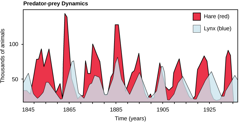
Consider the graph below, it depicts the relationship between the populations of Canadian lynx and snowshoe hare from North American forests. In this case, the Canadian lynx is the predator and snowshoe hare is the prey.

From this graph, we can infer that the population of Canadian lynx increased as the population of snowshoe hare rose. Similarly, the population of Canadian lynx dropped when the population of snowshoe hair decreased. It clearly states that the population of the two species is inter-dependent on each other.

This cycle of predator and prey lasts approximately 10 years, with the predator population lagging 1–2 years behind that of the prey population. As the population of prey grows, the predators can hunt more, hence the population of predators increases as well. When the population of predators reaches a threshold level, they kill a lot of prey, and thus the population of prey starts to decrease. This is followed by a decline in the predator population because of scarcity of food. When the predator population is low, the prey population starts to increase due, at least in part, to low predator pressure, starting the cycle anew.

Let’s try to visualize the predator-prey cycles.

Consider the scenario of fox versus rabbit. Here, fox is the predator and rabbit is the prey. Play with the sliders, to change the parameters of their relation, and see how the two populations are affected by each other. The values of the sliders below, are optimized for obtaining better graphs, with an initial rabbit population of 35 and initial fox population of 50.

There you have it. Hope the concept is more clear now!

Sources :

• Lotka–Volterra equations
• Alfred J. Lotka
• Vito Volterra
• Lotka-Volterra Equations
• Community Ecology
• Lotka-Volterra C++